Reading and writing data

A short description of the post.

Load R packages that we will need.

library(tidyverse)
library(here)
library(janitor)
library(skimr)

Download \(CO_2\) emissions per capita from Our World in Data into the directory for this post.

Assign the location of the file to file.csv. The data should be in the same directory as this file.

file_csv <- here("_posts",
              "2021-03-01-reading-and-writing-data",
              "co-emissions-per-capita.csv")
emissions <- read_csv(file_csv)

Show the first ten rows (observations of) emissions.
```
emissions
```

# A tibble: 22,383 x 4
   Entity      Code   Year `Per capita CO2 emissions`
   <chr>       <chr> <dbl>                      <dbl>
 1 Afghanistan AFG    1949                    0.00191
 2 Afghanistan AFG    1950                    0.0109 
 3 Afghanistan AFG    1951                    0.0117 
 4 Afghanistan AFG    1952                    0.0115 
 5 Afghanistan AFG    1953                    0.0132 
 6 Afghanistan AFG    1954                    0.0130 
 7 Afghanistan AFG    1955                    0.0186 
 8 Afghanistan AFG    1956                    0.0218 
 9 Afghanistan AFG    1957                    0.0343 
10 Afghanistan AFG    1958                    0.0380 
# … with 22,373 more rows

Start with emissions data, Then use clean names from the janitor package to make the names easier to work with assign the output to tidy_emissions show the first ten rows of tidy_emissions
```
tidy_emissions <- emissions %>% 
  clean_names()
tidy_emissions
```

# A tibble: 22,383 x 4
   entity      code   year per_capita_co2_emissions
   <chr>       <chr> <dbl>                    <dbl>
 1 Afghanistan AFG    1949                  0.00191
 2 Afghanistan AFG    1950                  0.0109 
 3 Afghanistan AFG    1951                  0.0117 
 4 Afghanistan AFG    1952                  0.0115 
 5 Afghanistan AFG    1953                  0.0132 
 6 Afghanistan AFG    1954                  0.0130 
 7 Afghanistan AFG    1955                  0.0186 
 8 Afghanistan AFG    1956                  0.0218 
 9 Afghanistan AFG    1957                  0.0343 
10 Afghanistan AFG    1958                  0.0380 
# … with 22,373 more rows

Start with the tidy_emissions THEN -use filter to extract rows with year == 2000 THEN -use skim to calculate the descriptive statistics.
```
tidy_emissions %>% 
  filter(year == 2000) %>% 
  skim()
```

Table 1: Data summary
Name	Piped data
Number of rows	219
Number of columns	4
_______________________
Column type frequency:
character	2
numeric	2
________________________
Group variables	None

Variable type: character

skim_variable	n_missing	complete_rate	min	max	empty	n_unique	whitespace
entity	0	1.00	4	32	0	219	0
code	12	0.95	3	8	0	207	0

Variable type: numeric

skim_variable	n_missing	complete_rate	mean	sd	p0	p25	p50	p75	p100	hist
year	0	1	2000.00	0.00	2e+03	2000.00	2000.00	2000.00	2000.00	▁▁▇▁▁
per_capita_co2_emissions	0	1	5.06	6.74	2e-02	0.71	2.82	7.97	58.39	▇▁▁▁▁

13 observations have a missing code. How are these observations different? -start with tidy_emissions then extract rows with year == 2000 and are missing a code.
```
tidy_emissions %>% 
  filter(year == 2000, is.na(code))
```

# A tibble: 12 x 4
   entity                     code   year per_capita_co2_emissions
   <chr>                      <chr> <dbl>                    <dbl>
 1 Africa                     <NA>   2000                     1.11
 2 Asia                       <NA>   2000                     2.40
 3 Asia (excl. China & India) <NA>   2000                     3.35
 4 EU-27                      <NA>   2000                     8.46
 5 EU-28                      <NA>   2000                     8.61
 6 Europe                     <NA>   2000                     8.48
 7 Europe (excl. EU-27)       <NA>   2000                     8.47
 8 Europe (excl. EU-28)       <NA>   2000                     8.19
 9 North America              <NA>   2000                    14.6 
10 North America (excl. USA)  <NA>   2000                     5.39
11 Oceania                    <NA>   2000                    12.6 
12 South America              <NA>   2000                     2.32

Start with tidy_emissions THEN -use filter -use select change the year -use remane to change entity to country -assign the output to emissions_2019

emissions_2000 <- tidy_emissions %>% 
  filter(year == 2000,!is.na(code)) %>%
  select(-year) %>% 
  rename(country = entity)

Which 15 countries have the highest per_capita_co2_emissions -start with emissions_2019 then -use slice_max -assign output to max_15_emitters
```
max_15_emitters <- emissions_2000 %>% 
  slice_max(per_capita_co2_emissions, n=15)
```

Which 15 countries have the lowest per_capita_co2_emissions? -start with emissions_2019 then -use slice_min -assign output to min_15_emitters
```
min_15_emitters <- emissions_2000 %>% 
  slice_min(per_capita_co2_emissions, n=15)
```

Use bind_rows to bind together the max_15_emitters and min_15_emitters -assign the output to max_min_15
```
max_min_15 <- bind_rows(max_15_emitters,min_15_emitters)
```

Export max_min_15 to 3 file formats.

max_min_15 %>% write_csv("max_min_15.csv") # comma-separated values
max_min_15 %>% write_tsv("max_min_15.tsv") # tab separated
max_min_15 %>% write_delim("max_min_15.psv",delim = "1") #pipe-separated

Read the 3 file formats into R

max_min_15.csv <- read_csv("max_min_15.csv") # comma-separated values
max_min_15.tsv <- read_tsv("max_min_15.tsv") # tab separated
max_min_15.psv <- read_delim("max_min_15.psv",delim = "1") # pipe-separated

Use setdiff to check for any differences among max_min_15.csv,max_min_15.tsv,max_min_15.psv
```
setdiff(max_min_15.csv,max_min_15.tsv,max_min_15.psv)
```

# A tibble: 0 x 3
# … with 3 variables: country <chr>, code <chr>,
#   per_capita_co2_emissions <dbl>

Reorder data

max_min_15_plot_data <- max_min_15 %>% 
  mutate(country = reorder(country, per_capita_co2_emissions))

Plot max_min_15_plot_data

ggplot(data = max_min_15_plot_data, aes(x= per_capita_co2_emissions, y= country)) +
            geom_col(fill = "blue", stat = "identity") +
            labs(title = "The top 15 and bottom 15 per capita CO2 emissions",
     subtitle = "for 2000",
     x= NULL, y= NULL)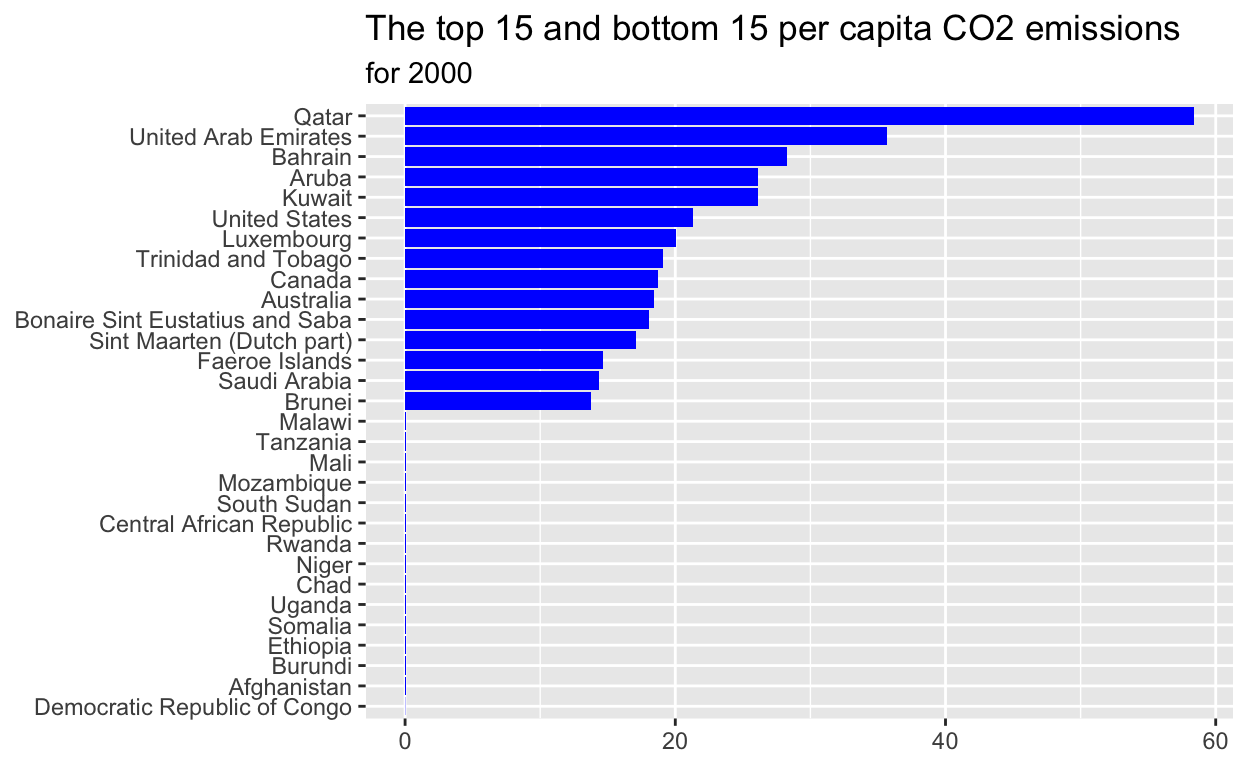

Save the plot directory with this post.

ggsave(filename = "preview.png", path = here("_posts","2021-03-01-reading-and-writing-data"))

Add preview.png to yaml